Reliable and reproducible statements on particle shape and size are essential
Images are beautiful. Images are intuitive. Images are meaningful. These are already some of the main advantages of Dynamic Image Analysis. But first things first.
Two recurrent tasks in particle analysis are the determination of the particle size distribution of a sample and questions about the shape of the particles. However, like so often, the selection of the appropriate method to accomplish these tasks depends on numerous parameters. And there is not always a clear answer as to which is the best method to cover all aspects of the task at hand as completely and efficiently as possible. The world is complex.
Thus, you first have to look at the essential characteristics of the material to be investigated and further clearly define what exactly the analysis should yield. And certainly the most important, central parameter here is simply the size of the particles to be examined: If these have a size of only a few micrometers and less, one will resort to other methods than with large chunks, which can also be several millimeters in size. Today, we will focus precisely on these "chunks", the range between a few micrometers and a few millimeters or even centimeters. This is the range in which images captured by light optics can show their strengths.
Dynamic Image Analysis – How does it work?
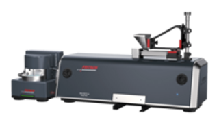
The ANALYSETTE 28 ImageSizer made by FRITSCH GmbH delivers such images, a whole flood of images. To be specific, up to about 75 images per second, and this at an image resolution of 5 mega pixels. These images are captured as the sample material passes the camera optics in the focal plane and is simultaneously illuminated using a backlight method. How exactly the particles are transported past the camera can be realized in different ways. In the simplest case, the sample material ripples from a vibratory feeder and falls continuously past the camera. Alternatively, however, the sample can be transferred to a suspension, which is then pumped through a measuring cell positioned in the focal plane of the camera optics. Both methods have their advantages, but also their limitations.
So, what do you do now with the captured images?
First, the software must detect each particle. To do this, the parts of the image that are darker than the background, the shadow of each particle, is searched for. You have to be aware that the camera does not only deliver either black or white pixels, but also numerous gray values in between. And at the particle edges the brightness transition from light to dark is not abrupt. Thus, it is necessary to determine starting from which gray value a pixel is identified as belonging to the particle, i.e. a threshold is introduced that divides all images into "particle" and "background". This process is called binarization. By the way, it is helpful if you can see in the software where exactly this binarization threshold is located on captured images. This gives you an important and helpful tool for judging how "reasonably" the software captures individual particles.
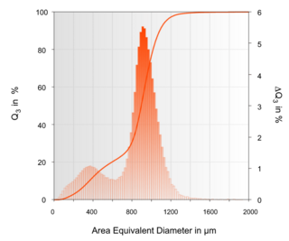
Once the binarization has taken place, numerous parameters are then determined from the obtained outlines for each detected particle. Unlike many other methods in particle size measurement, the user has a choice here: For irregularly shaped particles, you first need to think about the particle size definition to use. The ImageSizing Software (ISS) from Fritsch offers a wide range of possibilities here. Comparisons of distribution graphs using different definitions of particle size can then be made quickly and flexibly (Figure 2).
What can you find out about the shape of the individual particles?
In addition to determining the particle size distribution, Dynamic Image Analysis has a strong focus on shape detection, of course. How much do the particles of the examined sample deviate from the ideal spherical shape? What is the width-to-length ratio of the material? Do coarse particles differ fundamentally in shape from finer particles? These are just a few possible questions that can be addressed by an image acquisition system.
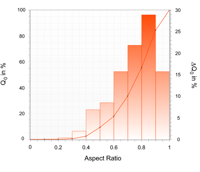
When displaying the shape parameters of an examined material sample, two different options are now available in the ImageSizing-Software ISS: For a selected shape parameter, e.g. the Aspect Ratio (width-to-length), a distribution analogous to a particle size distribution can be generated - instead of a particle size, the Aspect Ratio is plotted on the x-axis. The y-axis then represents either the relative fraction of particles with an Aspect Ratio smaller than the x-axis value (solid line in Figure 3, left y-axis) or the fraction within a certain Aspect Ratio interval (shown as a bar in Figure 3, right y-axis). This provides a quick, compact overview with respect to the selected shape parameter.
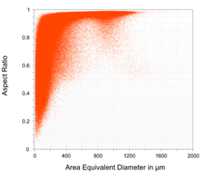
However, this representation does not show for which particle sizes certain Aspect Ratio values may occur preferentially, e.g. whether large particles tend to deviate from the perfect spherical shape more than smaller ones. This is where displaying the data in a 2D or even 3D Cloud is helpful. As an example, Figure 4 shows the same measurement as a 2D Cloud. Each measured particle generates a data point where the y value gives the Aspect Ratio and for x value the Area Equivalent Diameter is chosen. Of course, any other size (or even shape) parameter can also be used for the x axis.
It is obvious that for this example the smaller particles deviate more often from the spherical shape than the larger ones. However, we can also find a range around 750 µm particle size, where particles with a smaller aspect ratio also occur more frequently.
Conclusion
Let's return to the statement we made at the beginning: images are beautiful. Images are intuitive. Images are expressive. In a nutshell, this describes the great charm of the method. With many other techniques for particle sizing, you are facing something like a black-box approach. You throw in a sample, data is generated in an almost miraculous way, and a result appears at the end in the output box. A deeper understanding is usually possible, but involves considerable effort. Different here: You can always take a look at the images! And there you go, you can explain the result just by watching. Just like so.
-
Download the FRITSCH-report as PDF file

FRITSCH GmbH - Milling and Sizing
55743 Idar-Oberstein